19. Posterior Distributions for AR(1) Parameters#
GPU
This lecture was built using a machine with the latest CUDA and CUDANN frameworks installed with access to a GPU.
To run this lecture on Google Colab, click on the “play” icon top right, select Colab, and set the runtime environment to include a GPU.
To run this lecture on your own machine, you need to install the software listed following this notice.
In addition to what’s included in base Anaconda, we need to install the following package:
!pip install numpyro
We’ll begin with some Python imports.
import numpyro
from numpyro import distributions as dist

import jax.numpy as jnp
from jax import random, lax
import matplotlib.pyplot as plt
This lecture uses Bayesian methods offered by numpyro to make statistical inferences about two parameters of a univariate first-order autoregression.
The model is a good laboratory for illustrating the consequences of alternative ways of modeling the distribution of the initial \(y_0\):
As a fixed number
As a random variable drawn from the stationary distribution of the \(\{y_t\}\) stochastic process
The first component of the statistical model is
where the scalars \(\rho\) and \(\sigma_x\) satisfy \(|\rho| < 1\) and \(\sigma_x > 0\).
\(\{\epsilon_{t+1}\}\) is a sequence of i.i.d. normal random variables with mean \(0\) and variance \(1\).
The second component of the statistical model is
Consider a sample \(\{y_t\}_{t=0}^T\) governed by this statistical model.
The model implies that the likelihood function of \(\{y_t\}_{t=0}^T\) can be factored:
where we use \(f\) to denote a generic probability density.
The statistical model (19.1)-(19.2) implies
We want to study how inferences about the unknown parameters \((\rho, \sigma_x)\) depend on what is assumed about the parameters \(\mu_0, \sigma_0\) of the distribution of \(y_0\).
Below, we study two widely used alternative assumptions:
\((\mu_0,\sigma_0) = (y_0, 0)\) which means that \(y_0\) is drawn from the distribution \({\mathcal N}(y_0, 0)\); in effect, we are conditioning on an observed initial value.
\(\mu_0,\sigma_0\) are functions of \(\rho, \sigma_x\) because \(y_0\) is drawn from the stationary distribution implied by \(\rho, \sigma_x\).
Note
We do not treat a third possible case in which \(\mu_0,\sigma_0\) are free parameters to be estimated.
Unknown parameters are \(\rho, \sigma_x\).
We have independent prior probability distributions for \(\rho, \sigma_x\).
We want to compute a posterior probability distribution after observing a sample \(\{y_{t}\}_{t=0}^T\).
The notebook uses numpyro to compute a posterior distribution of \(\rho, \sigma_x\).
We will use NUTS samplers to generate samples from the posterior in a chain.
NUTS is a form of Monte Carlo Markov Chain (MCMC) algorithm that bypasses random walk behavior and allows for faster convergence to a target distribution.
This not only has the advantage of speed, but also allows complex models to be fitted without having to employ specialized knowledge regarding the theory underlying those fitting methods.
Thus, we explore consequences of making these alternative assumptions about the distribution of \(y_0\):
A first procedure is to condition on whatever value of \(y_0\) is observed.
This amounts to assuming that the probability distribution of the random variable \(y_0\) is a Dirac delta function that puts probability one on the observed value of \(y_0\).
A second procedure assumes that \(y_0\) is drawn from the stationary distribution of a process described by (19.1) so that \(y_0 \sim {\mathcal{N}} \left(0, \frac{\sigma_x^2}{(1-\rho)^2} \right)\)
When the initial value \(y_0\) is far out in the tail of the stationary distribution, conditioning on an initial value gives a posterior that is more accurate in a sense that we’ll explain.
Basically, when \(y_0\) happens to be in the tail of the stationary distribution and we don’t condition on \(y_0\), the likelihood function for \(\{y_t\}_{t=0}^T\) adjusts the posterior distribution of the parameter pair \(\rho, \sigma_x\) to make the observed value of \(y_0\) more likely than it really is under the stationary distribution, thereby adversely twisting the posterior in short samples.
An example below shows how not conditioning on \(y_0\) adversely shifts the posterior probability distribution of \(\rho\) toward larger values.
We begin by solving a direct problem that simulates an AR(1) process.
How we select the initial value \(y_0\) matters:
If we think \(y_0\) is drawn from the stationary distribution \({\mathcal N}(0, \frac{\sigma_x^{2}}{1-\rho^2})\), then it is a good idea to use this distribution as \(f(y_0)\).
Why? Because \(y_0\) contains information about \(\rho, \sigma_x\).
If we suspect that \(y_0\) is far in the tail of the stationary distribution – so that variation in early observations in the sample has a significant transient component – it is better to condition on \(y_0\) by setting \(f(y_0) = 1\).
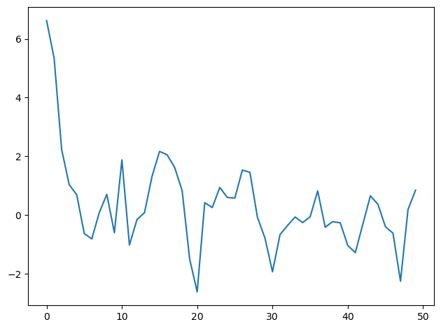
To illustrate the issue, we’ll begin by choosing an initial \(y_0\) that is far out in the tail of the stationary distribution.
def ar1_simulate(ρ, σ, y0, T, key):
    ε = random.normal(key, shape=(T,)) * σ

    def scan_fn(y_prev, ε_t):
        y_t = ρ * y_prev + ε_t
        return y_t, y_t

    _, y = lax.scan(scan_fn, y0, ε)

    return y

σ = 1.0
ρ = 0.5
T = 50

key = random.PRNGKey(0)
y = ar1_simulate(ρ, σ, 10.0, T, key)
plt.plot(y)
plt.tight_layout()
Now we shall use Bayes’ law to construct a posterior distribution, conditioning on the initial value of \(y_0\).
(Later we’ll assume that \(y_0\) is drawn from the stationary distribution, but not now.)
19.1. Implementation#
First, we’ll implement the AR(1) model conditioning on the initial value using numpyro.
The NUTS sampler is used to generate samples from the posterior distribution
def plot_posterior(sample):
    """
    Plot trace and histogram
    """
    ρs = sample['ρ']
    σs = sample['σ']

    fig, axs = plt.subplots(2, 2, figsize=(17, 6))

    # Plot trace
    axs[0, 0].plot(ρs)   # ρ
    axs[1, 0].plot(σs)   # σ

    # Plot posterior
    axs[0, 1].hist(ρs, bins=50, density=True, alpha=0.7)
    axs[0, 1].set_xlim([0, 1])
    axs[1, 1].hist(σs, bins=50, density=True, alpha=0.7)

    # Set axis labels for clarity
    axs[0, 0].set_ylabel("ρ")
    axs[0, 1].set_xlabel("ρ")
    axs[1, 0].set_ylabel("σ")
    axs[1, 1].set_xlabel("σ")

    # Unify the y-axis limits for trace plots
    max_ylim = max(axs[0, 0].get_ylim()[1], axs[1, 0].get_ylim()[1])
    axs[0, 0].set_ylim(0, max_ylim)
    axs[1, 0].set_ylim(0, max_ylim)

    # Unify the x-axis limits for histograms
    max_xlim = max(axs[0, 1].get_xlim()[1], axs[1, 1].get_xlim()[1])
    axs[0, 1].set_xlim(0, max_xlim)
    axs[1, 1].set_xlim(0, max_xlim)

    plt.tight_layout()
    plt.show()
def AR1_model(data):
    # Set prior
    ρ = numpyro.sample('ρ', dist.Uniform(low=-1., high=1.))
    σ = numpyro.sample('σ', dist.HalfNormal(scale=jnp.sqrt(10)))

    # Expected value of y in the next period (ρ * y)
    yhat = ρ * data[:-1]

    # Likelihood of the actual realization
    numpyro.sample('y_obs',
                dist.Normal(loc=yhat, scale=σ), obs=data[1:])
y = jnp.array(y)

# Set NUTS kernel
NUTS_kernel = numpyro.infer.NUTS(AR1_model)

# Run MCMC
mcmc = numpyro.infer.MCMC(NUTS_kernel,
            num_samples=50000, num_warmup=10000, progress_bar=False)
mcmc.run(rng_key=random.PRNGKey(1), data=y)
plot_posterior(mcmc.get_samples())
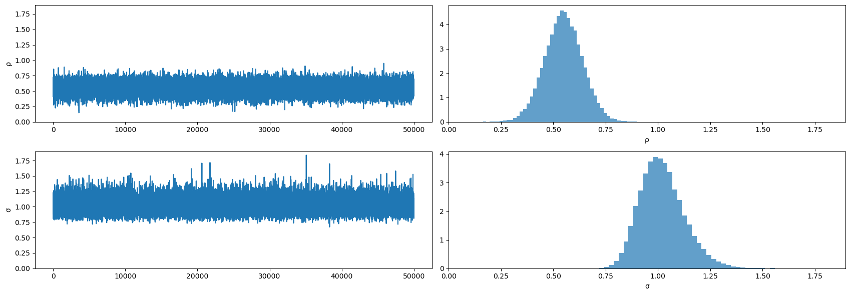
Evidently, the posteriors aren’t centered on the true values of \(.5, 1\) that we used to generate the data.
This is a symptom of the classic Hurwicz bias for first order autoregressive processes (see [Hurwicz, 1950].)
The Hurwicz bias is worse the smaller is the sample (see [Orcutt and Winokur, 1969]).
Be that as it may, here is more information about the posterior.
mcmc.print_summary()
                mean       std    median      5.0%     95.0%     n_eff     r_hat
         ρ      0.55      0.09      0.55      0.40      0.70  32204.63      1.00
         σ      1.02      0.11      1.01      0.85      1.19  33033.40      1.00

Number of divergences: 0
Now we shall compute a posterior distribution after seeing the same data but instead assuming that \(y_0\) is drawn from the stationary distribution.
This means that
Here’s the new code to achieve this.
def AR1_model_y0(data):
    # Set prior
    ρ = numpyro.sample('ρ', dist.Uniform(low=-1., high=1.))
    σ = numpyro.sample('σ', dist.HalfNormal(scale=jnp.sqrt(10)))

    # Standard deviation of ergodic y
    y_sd = σ / jnp.sqrt(1 - ρ**2)

    # Expected value of y in the next period (ρ * y)
    yhat = ρ * data[:-1]

    # Likelihood of the actual realization
    numpyro.sample('y_obs',
                    dist.Normal(loc=yhat, scale=σ), obs=data[1:])
    numpyro.sample('y0_obs',
                    dist.Normal(loc=0., scale=y_sd), obs=data[0])
y = jnp.array(y)

# Set NUTS kernel
NUTS_kernel = numpyro.infer.NUTS(AR1_model_y0)

# Run MCMC
mcmc2 = numpyro.infer.MCMC(NUTS_kernel,
                num_samples=50000, num_warmup=10000, progress_bar=False)
mcmc2.run(rng_key=random.PRNGKey(1), data=y)
plot_posterior(mcmc2.get_samples())
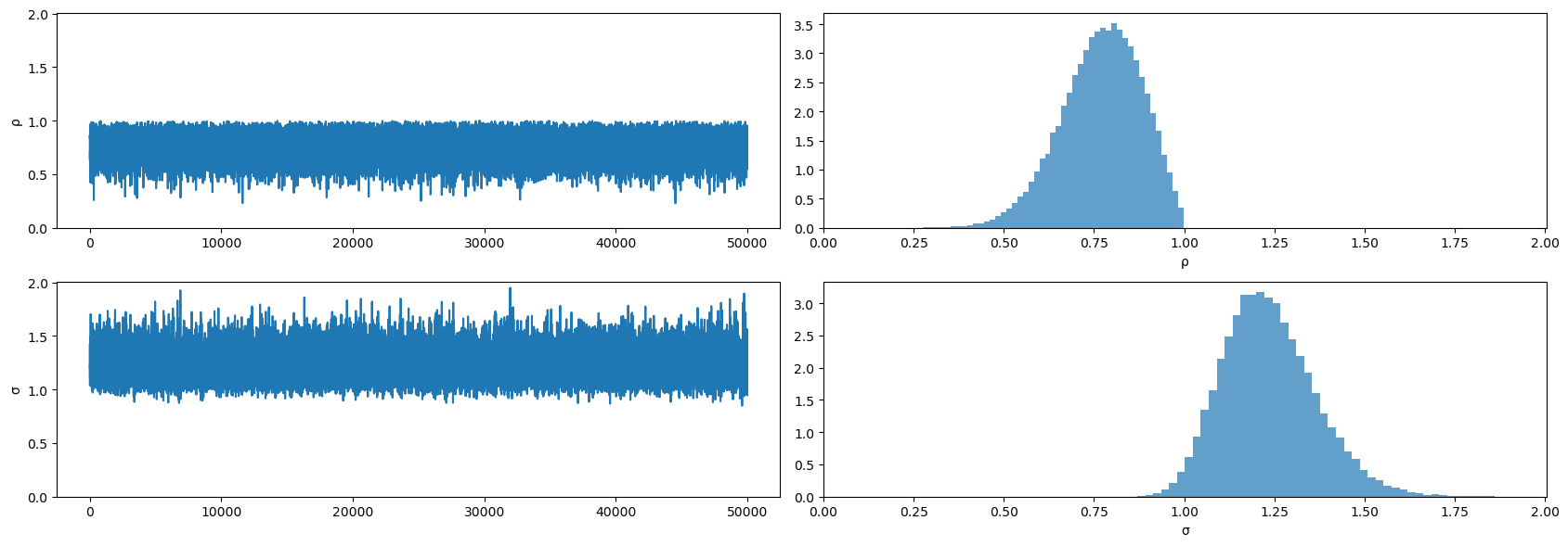
mcmc2.print_summary()
                mean       std    median      5.0%     95.0%     n_eff     r_hat
         ρ      0.77      0.11      0.78      0.60      0.95  25754.51      1.00
         σ      1.24      0.13      1.23      1.03      1.44  26869.58      1.00

Number of divergences: 0
Please note how the posterior for \(\rho\) has shifted to the right relative to when we conditioned on \(y_0\) instead of assuming that \(y_0\) is drawn from the stationary distribution.
Think about why this happens.
Hint
It is connected to how Bayes Law (conditional probability) solves an inverse problem by putting high probability on parameter values that make observations more likely.
Look what happened to the posterior!
It has moved far from the true values of the parameters used to generate the data because of how Bayes’ Law (i.e., conditional probability)
is telling numpyro to explain what it interprets as “explosive” observations early in the sample.
Bayes’ Law is able to generate a plausible likelihood for the first observation by driving \(\rho \rightarrow 1\) and \(\sigma \uparrow\) in order to raise the variance of the stationary distribution.
Our example illustrates the importance of what you assume about the distribution of initial conditions.